APGEOG4440 M - Geoinformatics Remote Sensing II (Winter 2015-2016)
Road Enhancement
After generating the resultant noise-reduced image, roads were enhanced and then separated from the background in order to prepare for the actual roads extraction later on. Before performing enhancement (calculation in Raster calculation), a low pass filtered image (3x3), or a fuzzy image in other words, of corrected band 3 (with both FME and MNFNR) was created by Averaging Mean Filter (FAV).
By looking up in Geomatica Online Help, FAV is an algorithm which performs average filtering on image data. The image data will be smoothed and noise will be suppressed as well after processing. The purpose of it was to emphasize on larger homogenous areas with similar pixel values and to reduce smaller details in the image. The Algorithm Library was opened and FAV was selected under 'All Algorithms'. After that, FAV Module Control panel was popped up. Corrected band 3 image was selected as 'Input: Unfiltered Layer'. 'Input Params 1' was kept as default of which both 'Filter X Size (Pixels)' and 'Filter Y Size (Pixels)' were 3 (i.e. 3x3 Filter). The output of this function was saved within the newly merged dataset for further manipulation. After running the function, the corrected image was viewed in Geomatica automatically.


From the comparison above, it is obvious that there is a loss of detail within the fuzzy image. It is more blurry and less clear than the corrected band 3 produced before. The contrast between urban areas and rural areas, such as the difference between roads and vegetations, is more outstanding.
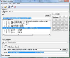
After performing FAV algorithm, calculation for enhancement was carried out. At the beginning, 3 new raster layers (8-bit channels) were created in preparation for the outputs (Files>New>Raster Layer). As mentioned in the guideline of this assignment, the enhancement equation is:
RED + [(RED-FUZZY)*X], {X = 2,8,16}
It means that this enhancement equation has to be performed for 3 times separately at a scaling factor of 2, 8 and 16 respectively. In 'Raster Calculator', this equation was inputted:
%2+((%2-%6)*X), {X = 2,8,16}
These 3 different outputs were saved in the newly created 8-bit channels one by one. And the 3 scaling maps are presented in grey scale as below.


From these 3 images, it is observed that the features with similar reflectance values are clustered and become more outstanding. For example, the pixel values of roads become higher (brighter) and easier to distinguish from other features, such as vegetation cover with lower values (darker). This contrast becomes more and more obvious from scaling factor 2, 8, to 16. The histograms for the 3 scaling factors are shown below.


By looking at these 3 histograms, one of the common points is that the pixel values have made use of the full radiometric range (i.e. 0-255). Pixels with similar values are clustered and form a several pikes in the histograms. The distance between these pikes becomes farther and farther when reaching a higher scaling factor of enhancement. The number of pixels with the value of 255 is increasing gradually relative to the rise in scaling factor. Again, it is commonly known that the pixel values of paved roads or other urban features are relative higher than the non-urban features'. Therefore, from these results, we can conclude that such enhancement can make different features more outstanding and easier to separate from the others. The contrast between different features is more prominent with a higher scaling factor enhancement. As a result, the enhancement with the scaling factor of 16 was selected for further extraction due to the great contrast between road features and background features.
In order to make a better comparison between these 3 scaling factors, 3 true-color and 3 false-color images are prepared. To create the true-color images, corrected band 3 (Enhancement x2, x8 & x16), corrected band 2 and corrected band 1 were assigned to red, green and blue channels respectively. To create the false-color images, original band 4 (NIR), corrected band 3 (Enhancement x2, x8 & x16) and corrected band 2 were assigned to red, green and blue channels respectively. Linear enhancement was applied to all images for better presentation.
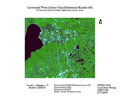


From the true-color images, we can see that there is a blue tint covering the image when it is compared to the true-color map produced in section 2. This impact is more obvious over the urban features. One of the possible reasons is that the filter algorithms applied to the original bands 1, 2 and 3 have altered the data. For example, the data might become biased towards NIR and SWIR data values when MNFNR utilized original bands 4 and 5 as inputs. We can also see that the contrast between road and non-road features increases when the scaling factor for enhancement increases. This contrast is the most obvious in the image with the scaling factor of 16.


From the false-color images, we can get a similar conclusion that the contrast between road and non-road features becomes more outstanding when the scaling factor increases. However, the level of noise has also increased with the rising scaling factor. It is especially obvious above the lake in the western area of the maps.
Please Click Image to Enlarge!